A connection between the Markov and Laplace matrix from the lens of the Gershgorin disk theorem

Introduction

Mathematics is all about connections. In this post I want to share with you a starkingly beautiful connection between the Markov and graph Laplacian matrix. This was the result of trying to find a fast algorithm to visualize data that preserves certain nice properties of the underlying space. In a moment of eureka I payed closer attention to this connection and found that all I needed for my problem was an application of the Gershgorin domain theorem. This connection came some time after writing my previous post so I thought it would be a good follow-up.

I would’ve liked to have written a short paper about this discovery, but this connection had already been reported in the literature in 2014 by the title Diverse Power Iteration Embeddings and Its Applications by Huang et al. Since I cannot write a paper on it, I’ll indulge myself in the pleasure of explaining the discovery in plain and hopefully intuitive language.

Motivation and rationale: data visualization and clustering

I was using a lot the Laplacian Embedding in my research in order to visualize data. In a nutshell, the algorithm works by finding the smallest eigenvectors associated with the smallest (non-zero) eigenvalues of the Laplacian matrix or graph Laplacian Matrix (we’ll get to the definition in a moment). This matrix is square and has number of rows and columns being equal to the number of datapoints. If you have millions or billions of datapoints, you can imagine that finding the eigenvectors of this matrix can be computationally expensive. I thought to myself that it was a waste of computation to get all of the eigenvectors–since all we need is the first three or so in order to visualize data, and at most on the order of hundreds if we needed to use it for clustering. This started my quest to finding a faster algorithm.

At first I thought of using the Power method - since the flavor of the problem was a good fit. However, the power method is used for the largest eigenpairs - and remember we want the smaller vectors of the spectrum. This led me to the inverse power method which is explained in the classic Linear Algebra book by Gilbert Strang. However, I was not satisfied by this approach and remembered that in the classic Spectral clustering tutorial paper by Ulrike von Luxburg, she mentions connections between the spectrum of different versions of the graph Laplacian, one of which is computed from a Markov matrix, that is the row stochastic matrix associated with a random walk on an undirected graph. In her paper, Von Luxburg mentions the connection that the largest eigenvalues of the Markov matrix correspond to the smallest of the random walk graph Laplacian but doesn’t prove it. The same is true for the study of Huang et al.

The above connection led me to try to prove this connection using the Gershgorin domain theorem.

Preliminaries

We start by using an adjacency matrix \(A\) that represents an undirected graph.

Definition Adjacency matrix \(A\). The construction for this matrix is straight-forward: it’s a binary symmetric matrix, with a 1 in the (i,j) position if node i is connected to node j. Thus, the adjacency matrix encodes the connectivity of a graph or network.

You can build this matrix from data using for example a k-nearest neighbors (kNN) approach.

Then, we need another very important matrix, the degree matrix \(D\) by summing across the rows of the adjacency matrix.

Definition Degree matrix.

The degree matrix is diagonal with \(D_{ii} = \sum_{j=1}^n A_{ij}\), where \(A\) is the adjacency matrix.

This matrix then represents the number of connections each node has.

We define the associated Markov matrix as follows:

Definition: Markov matrix. The Markov transition matrix for an undirected graph is defined as \(P = D^{-1}A\), where \(D\) is the degree matrix and \(A\) is the adjacency matrix. We denote it \(P\) as it is a probabilistic matrix. More specifically, using the (i,j) entry of \(P\) we get the probability of visiting each node \(j\) in the graph starting from node \(i\). In other words we get the dynamics of a random walk on the graph!

Definition: Random walk Laplacian

The random walk Laplacian is defined as:

\[\begin{align} L^{rw} = D^{-1}L = I - P \end{align}\]

where \(L = D - A\) is the unnormalized graph Laplacian. It turns out that the spectrum of \(L\) and \(L^{rw}\) coincide, as we’ll show in the next section.

With these ingredients and with the definitions laid down in my previous post on the Gershgorin domain theorem we can get to the core of this post!

Theorems

Proposition Markov and Laplace eigenvectors coincide.

Proof: We show this for the case of the random walk Laplacian. We directly show this by expanding the eigenvector-eigenvalue relation of each of these matrices.

\[\begin{align} Lv = (I-P)v = v - Pv = \lambda v \\ \implies Pv = v - \lambda v \\ \implies Pv = (1 - \lambda)v \end{align}\]

More importantly the smallest eigenvalue of the Laplacian is exactly the largest eigenvalue of the Markov as we show next. But first, we need to bound the eigenvalues of the Markov matrix since this will give us bounds on the Laplace spectrum - which is what we ultimately want.

Lemma: Markov spectrum is bounded to the unit disk of the complex plane.

Proof: This follows by application of the Gershgorin domain theorem. Since the rows sum to one, the radius of each Gershgorin disk cannot exceed the one. Let \(D_i\) be the i-th Gershgorin disk

• Case 1: If \(P_{ii} = 0 \implies D_i = B_{1}(0) \subset \mathbb{C}\), that is, if the diagonal entry \(i\) of the markov matrix is 0, then the sum of the off diagonal entries of the row sum to one and thus the corresponding Gershgorin disk is the unit closed ball centered at zero.
• Case 2: If \(P_{ii} = 1 \implies D_i = B_{0}(1)\)
• Case 3 (general case) : If \(P_{ii} \in (0,1) \implies D_i = B_x(y)\) where \(x + y = 1, x,y \in (0,1)\).

This concludes our proof.

Thus, we just showed that the magnitude of the eigenvalues of a Markov matrix is less than or equal to one, i.e. that the spectrum of a Markov matrix \(P\) is bounded to the unit disk of the complex plane.

We now bound the spectrum of the random walk graph Laplacian matrix.

Corollary \(\mathrm{spec} \, L^{rw} \subseteq 1 - \mathbb{D^2}\)

Proof: The proof is a straightforward calculation:

\[\begin{align} \lambda_L^{rw} &= 1 - \lambda_P \\ \implies \mathrm{spec} \, L^{rw} &\subseteq 1 - \mathrm{spec} \, P\\ &\subseteq 1 - \mathbb{D^2} \subseteq \mathbb{C} \end{align}\]

Geometric interpretation of the connection between the spectrum of Laplace and Markov matrices

It’s a good moment to step back and think about what we have just arrived and what are the consequences for our goal. For this, I’d like to bring some pictures to visualize our results.

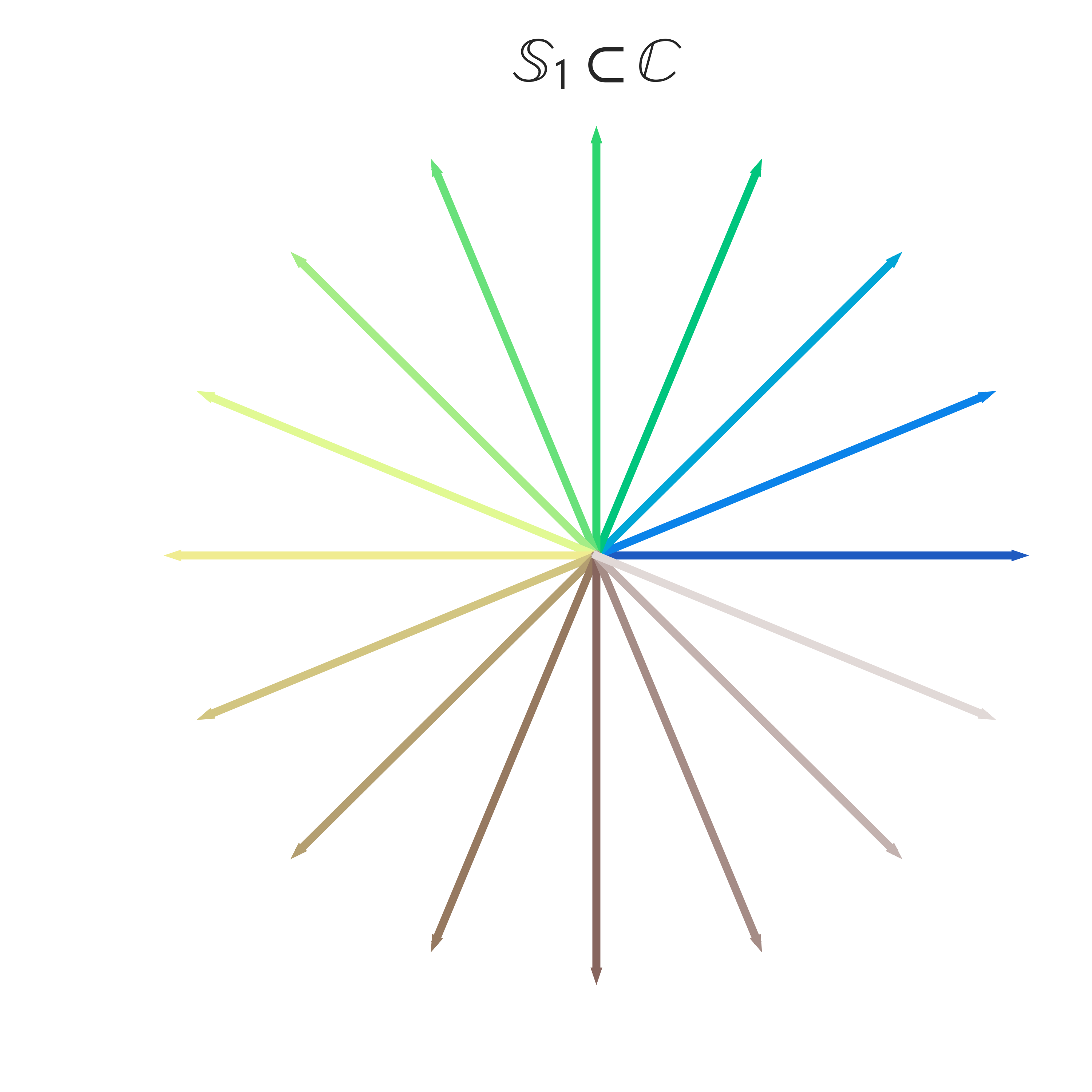
First, the Gershgorin disk theorem tells us that the spectrum of a Markov matrix lives in the unit disk. For visualization, let’s look at the vectors in the unit circle and color them by their angle.

But where does the spectrum of the Laplacian live in the complex plane?

We have the equation \(\lambda_L = 1 - \lambda_p\). This remarkably beautiful and simple formula puzzled me for a while, since written in set notation \(\mathrm{spec} \, L \subseteq 1 - \mathbb{D^2}\). Let’s break this down.

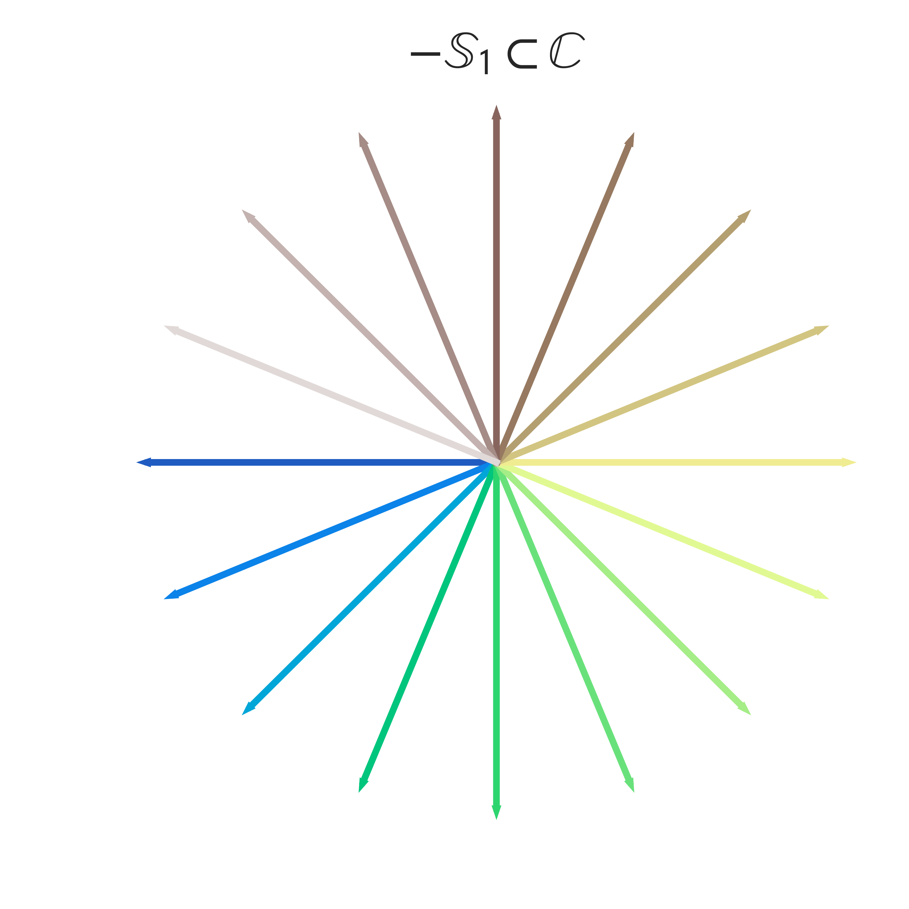
First, the negative of a complex number is just the negative of the real and the imaginary part. Thus we can think of multuplying a complex number by -1 as the action of the linear transformation \(\mathrm{diag}(-1,-1)\). We can visualize the operation of the negative of vectors in the complex unit circle as follows:

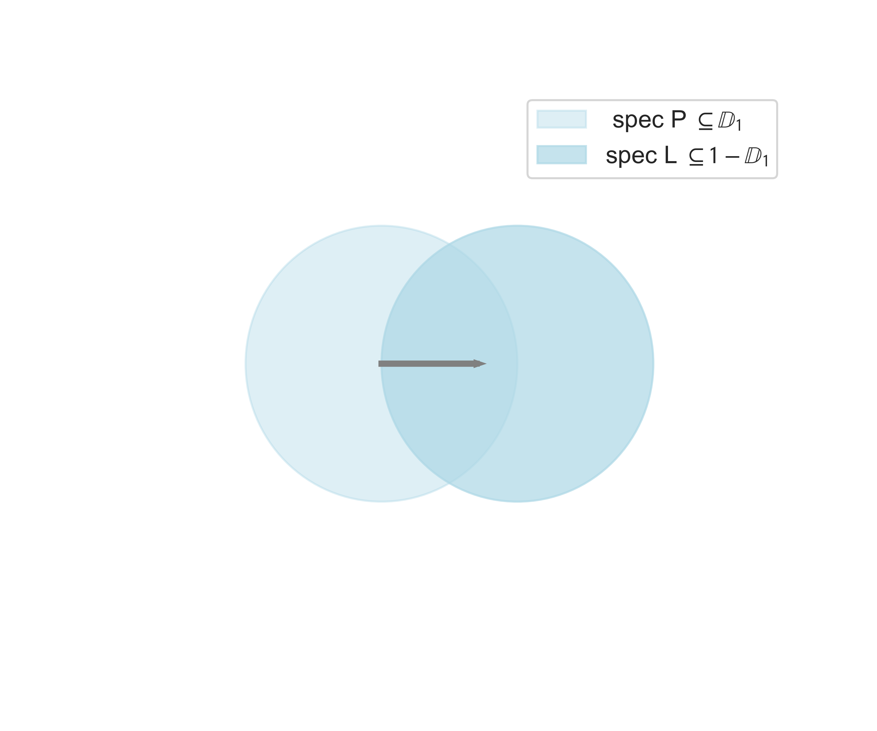
Finally, to get the set \(1 - \mathbb{D^2}\) we just need to shift the disk one unit to the right in the real component of the complex plane (horizontal direction). We can visualize the Gershgorin domains as follows (follow the colors to see where each original vector lands after the transformation!):

Importantly, let’s imagine following the eigenvalue 1 of Markov. Our formula tells us that the corresponding eigenvalue of the Laplace matrix would be zero! Geometrically, we first would have to multiply it by -1 which would flip it to the vector \((-1,0)^T\) in the complex plane and then shifting it to the right by a unit which would take it to the origin in the complex plane, i.e. the complex number 0.

If you’re following along, you can guess now where the largest eigenvalues of the Laplace matrix will land w.r.t. to the corresponding eigenvalues of its Markov matrix. Don’t worry if you don’t – the whole idea of dealing with the complex plane can be confusing. But it’s important to think about, as Markov matrices can indeed have imaginary eigenvalues.

Luckily for us we can bound the spectrum to the real numbers: it is a fact that if a matrix is symmetric by the Spectral theorem this implies that the eigenvalues of the matrix are real. Furthermore if a matrix is positive semidefinite its eigenvalues are non-negative. This is the last ingredient which helps us bound the eigenvalues of the Laplacian matrix and give a direct segway to our algorithm.

The final step : keeping it real

We now have an explicit bounding region for which the eigenvalues of the Laplacian live. Note that we have been working with the random walk Laplacian to make the connection to Markov matrices. We now define an alternative version of the graph Laplacian:

Definition The Symmetric graph Laplacian is defined as \(L^s = D^{-1/2} \, L \, D^{-1/2}\).

The above definition is helpful for inheriting the properties of a symmetric matrix, and especially for our discussion the fact that symmetric matrices have real eigenvalues. To see why this is important for us note that : \(D^{-1/2} \, ( L^s )\, D^{1/2} = D^{-1/2} \, ( D^{-1/2} \, L \, D^{-1/2}) \, D^{1/2} = D^{-1} \, L = L^{rw}\)

In fancy mathematical language this shows that the Symmetric graph Laplacian and the Random Walk Laplacian are similar. Thus, they have the same spectrum. This means that the eigenvalues of the Random Walk Laplacian are also all real, since the symmetric Laplacian has only real eigenvalues by the Spectral theorem.

This leads to the following refinement of our last corollary.

Corollary (refinement) \(\mathrm{spec} \, L^{rw} \subseteq [0,2]\)

Using this last statement, we can finally see why the largest eigenvalues of the Markov matrix correspond to the smallest eigenvalues of the Laplacian matrix. For the sake of our argument, let’s also focus on symmetrized markov matrices: \(P^{s} = \frac{1}{2} ( P + P^T)\). Using this construction, the spectrum of symmetric Markov matrices will be a subset of the interval \([-1,1] \subset \mathbb{R}\). We can now talk about smallest and largest in the ordering sense.

Using the equation \(\lambda_L = 1 - \lambda_P\), we can see that thinking of the spectrums as ordered sets, the negative sign flips the order of the eigenvalues from largest to smallest and viceversa, and then shifts the intervals by 1 to the right. It helped me to imagine doing the operation by having numpy arrays and imagine taking a linearly increasing sample of the interval \([-1,1]\) and then just applying our operation.

With this in mind, we can finally write down our algorithm for fast visualization using the Laplacian embedding.

Algorithm : Markov-Laplace embedding

1. Construct a graph from data, and store it in adjacency matrix \(A\).
2. Compute the Markov matrix \(P\) associated with \(A\).
3. Compute the first three largest eigenvectors of \(P\) using the Power method.
4. Discard the first one (associated with eigenvalue 1 of Markov).
5. Visualize data in vectors 2 and 3.

This is a fast method to visualize data using the Laplacian Embedding. If you set a random seed, then your embeddings will be deterministic. Enjoy!

The Laplacian matrix and connections to other concepts in math

The Laplacian matrix is one of the mathematical objects which I’ve found to have some of the most fascinating connections to different geometrical and physical phenomena. These are some of my favorite:

• The solutions of the heat equation in a graph

• Hearing the shape of a drum (or can we?)

• Transferring the pose of an armadillo to Homer simpson.

Final note : alternative proof for the upper bound on the eigenvalues of the Laplacian graph

Not too long ago (at most a couple of years) I came across the classic notes of Spectral Graph Theory from Fan Chung, and I remember not being able to follow the proof for the Lemma 1.7(v) that states essentially that the eigenvalues of the graph Laplacian are smaller than or equal to 2. This is an alternative proof for that statement using a different approach.

To see this note that our proof focused on the random walk Laplacian, but the eigenvalues coincide with those of the classic graph Laplacian.

Acknowledgements

I’d like to especially thank to my advisor Matt Thomson for introducing me into the rigor of mathematics and particularly the appreciation of Linear Algebra.

Secondly, I am massively grateful to Kostia Zuev for his lectures on Applied Linear Algebra. This post is a direct consequence of taking his course, ACM 104.

Finally, I’d like to thank my friend and collaborator Alejandro Granados. This idea was developed while working under his supervision at the CZ Biohub Summer Internship in Angela Pisco’s Data Science team.